
图像算法代写|ECE 232E Project 4 Graph Algorithms
这是一个图像算法相关的CS代写案例
Introduction
In this project we will explore graph theory theorems and algorithms, by applying them on real data. In the first part of the project, we consider a particular graph modeling correlations between stock price time series. In the second part, we analyse traffic data on a dataset provided by Uber. Third part of the project asks you to define your own task.
Fourth part of the project is related to shortest paths, and is UNGRADED, OPTIONAL. However, it is suggested that you complete it before finishing part, especially if you struggle with the runtimes for questions 19-24.
1. Stock Market
In this part of the project, we study data from stock market. The data is available on this Dropbox Link. The goal of this part is to study correlation structures among fluctuation patterns of stock prices using tools from graph theory. The intuition is that investors will have similar strategies of investment for stocks that are effected by the same economic factors. For example, the stocks belonging to the transportation sector may have different absolute prices, but if for example fuel prices change or are expected to change significantly in the near future, then you would expect the investors to buy or sell all stocks similarly and maximize their returns. Towards that goal, we construct different graphs based on similarities among the time series of returns on different stocks at different time scales (day vs a week). Then, we study properties of such graphs. The data is obtained from Yahoo Finance website for 3 years. You’re provided with a number of csv tables, each containing several fields: Date, Open, High, Low, Close, Volume, and Adj Close price. The files are named according to Ticker Symbol of each stock. You may find the market sector for each company in Name sector.csv. We recommend doing this part of the project (Q1 – Q8) in R.
1. Return correlation
In this part of the project, we will compute the correlation among log-normalized stock-return time series data. Before giving the expression for correlation, we introduce the following nota- tion:
![]()
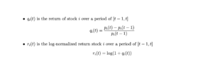
Then with the above notation, we define the correlation between the log-normalized stock-return time series data of stocks i and j as
![]()
where ⟨·⟩ is a temporal average on the investigated time regime (for our data set it is over 3 years).
QUESTION 1: What are upper and lower bounds on ρij? Provide a justification for using log- normalized return (ri(t)) instead of regular return (qi(t)).
2. Constructing correlation graphs
In this part,we construct a correlation graph using the correlation coefficient computed in the previous section. The correlation graph has the stocks as the nodes and the edge weights are given by the following expression
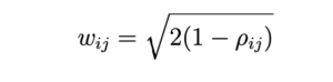
Compute the edge weights using the above expression and construct the correlation graph.
QUESTION 2: Plot a histogram showing the un-normalized distribution of edge weights.
3. Minimum spanning tree (MST)
In this part of the project, we will extract the MST of the correlation graph and interpret it.
QUESTION 3: Extract the MST of the correlation graph. Each stock can be categorized into a sector, which can be found in Name sector.csv file. Plot the MST and color-code the nodes based on sectors. Do you see any pattern in the MST? The structures that you find in MST are called Vine clusters. Provide a detailed explanation about the pattern you observe.
QUESTION 4: Run a community detection algorithm (for example walktrap) on the MST ob- tained above. Plot the communities formed. Compute the homogeneity and completeness of the clustering. (you can use the ’clevr’ library in r to compute homogeneity and completeness).
4. Sector clustering in MST’s
In this part, we want to predict the market sector of an unknown stock. We will explore two methods for performing the task. In order to evaluate the performance of the methods we define the following metric

where Si is the sector of node i. Define
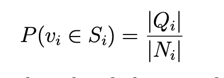
where Qi is the set of neighbors of node i that belong to the same sector as node i and Ni is the set of neighbors of node i. Compare α with the case where
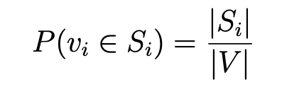
QUESTION 5: Report the value of α for the above two cases and provide an interpretation for the difference.
5. Correlation graphs for weekly data
In the previous parts, we constructed the correlation graph based on daily data. In this part of the project, we will construct a correlation graph based on WEEKLY data. To create the graph, sample the stock data weekly on Mondays and then calculate ρij using the sampled data. If there is a holiday on a Monday, we ignore that week. Create the correlation graph based on weekly data.
QUESTION 6: Repeat questions 2,3,4,5 on the WEEKLY data.
6. Correlation graphs for MONTHLY data
In this part of the project, we will construct a correlation graph based on MONTHLY data. To create the graph, sample the stock data Monthly on 15th and then calculate ρij using the sampled data. If there is a holiday on the 15th, we ignore that month. Create the correlation graph based on MONTHLY data.
QUESTION 7: Repeat questions 2,3,4,5 on the MONTHLY data.
QUESTION 8: Compare and analyze all the results of daily data vs weekly data vs monthly data. What trends do you find? What changes? What remains similar? Give reason for your observations. Which granularity gives the best results when predicting the sector of an unknown stock and why?
本网站支持淘宝 支付宝 微信支付 paypal等等交易。如果不放心可以用淘宝交易!
E-mail:itcsdx@outlook.com 微信:itcsdx
如果您使用手机请先保存二维码,微信识别。如果用电脑,直接掏出手机果断扫描。